Introduction
If you want to predict the amount of rainfall, yield crops, or other attribute , you may need to learn about the interpolation methods like inverse distance weighted (IDW).
IDW is a deterministic method for interpolation, once you have a set of know points, you can use IDW to estimate values for unknown points. For instance, you have 6 know points with rainfall attribute, and you need to predict the rainfall for a 7th point (Figure 1).

Figure 1: Know and Unknown points
The math behind Inverse Distance Weighting is simple. Just keep in mind that the search distance or number of closest points assigns how many points will be used to predict the unknown point, equation:
$$w(x)=\frac{A}{B}$$
$$A = \sum_{i=1}^{n} \frac{1}{d(x, x_i)^p}~ui$$
$$B = \sum_{i=1}^{n} \frac{1}{d(x, x_i)^p}$$
where: w is the predicted value, d is the distance, x is the unknown point,
x
Example using Pyhton
Check the know points. Notice that x and y are coordinates in degree:
| x | y | rain |
|---|---|---|
| -47.6 | -23.4 | 27 |
| -48.9 | -24 | 33.4 |
| -48.2 | -23.9 | 34.6 |
| -48.9 | -23.1 | 18.2 |
| -47.6 | -22.7 | 30.8 |
| -48.6 | -22.5 | 42.8 |
For Python we will make our own code. We need two functions, one of them for distances calculation, and another one to prediction.
# packages
import math
import numpy as np
#------------------------------------------------------------
# Distance calculation, degree to km (Haversine method)
def harvesine(lon1, lat1, lon2, lat2):
    rad = math.pi / 180  # degree to radian
    R = 6378.1  # earth average radius at equador (km)
    dlon = (lon2 - lon1) * rad
    dlat = (lat2 - lat1) * rad
    a = (math.sin(dlat / 2)) ** 2 + math.cos(lat1 * rad) * \
        math.cos(lat2 * rad) * (math.sin(dlon / 2)) ** 2
    c = 2 * math.atan2(math.sqrt(a), math.sqrt(1 - a))
    d = R * c
    return(d)
# ------------------------------------------------------------
# Prediction
def idwr(x, y, z, xi, yi):
    lstxyzi = []
    for p in range(len(xi)):
        lstdist = []
        for s in range(len(x)):
            d = (harvesine(x[s], y[s], xi[p], yi[p]))
            lstdist.append(d)
        sumsup = list((1 / np.power(lstdist, 2)))
        suminf = np.sum(sumsup)
        sumsup = np.sum(np.array(sumsup) * np.array(z))
        u = sumsup / suminf
        xyzi = [xi[p], yi[p], u]
        lstxyzi.append(xyzi)
    return(lstxyzi)
Solving:
# know points
x = [-47.6, -48.9, -48.2, -48.9, -47.6, -48.6]
y = [-23.4, -24.0, -23.9, -23.1, -22.7, -22.5]
z = [27.0,  33.4,  34.6,  18.2,   30.8, 42.8]
# unknow point
xi = [-48.0530600]
yi = [-23.5916700]
# running the function
idwr(x,y,z,xi,yi)
# output
[[-48.05306, -23.59167, 31.486682779040855]]
Plotting with distances (Figure 2):
import matplotlib.pyplot as plt
import matplotlib.style as style
style.available
style.use('seaborn-white')
dists = [50.93664088924365, 97.50798854810864, 37.44644402279387, 102.4130216426453, 109.55825855482198, 133.81580425549404]
len(dists)
for i in range(len(x)):
    plt.scatter(x = x[i],
                y = y[i],
                label=label[i],
                s = 50)
    plt.annotate(xy = (x[i],y[i]),
                 s=z[i])
    plt.annotate(xy = ( ((x[i] + xi[0]) / 2), ((y[i] + yi[0]) / 2)),
                 s= 'dist='+ str(np.round(dists[i],2))+ ' km')
    lcx = [xi[0], x[i]]
    lcy = [yi[0], y[i]]
    plt.plot(lcx,lcy)
plt.scatter(xi,yi,
            c='black', s=230, label='unknown', marker='*')
plt.legend(bbox_to_anchor=(1.04,1), loc="upper left")
plt.tight_layout()
plt.grid(True)
plt.show()
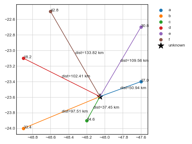
Figure 2: Know and Unknown points
Validation using R
library(gstat)
library(sp)
dfsp = data.frame(x = c(-47.6, -48.9, -48.2, -48.9, -47.6, -48.6),
                  y = c(-23.4, -24.0, -23.9, -23.1, -22.7, -22.5),
                  chuva = c(27.0,  33.4,  34.6,  18.2,   30.8, 42.8))
sp = dfsp
coordinates(sp) = ~x+y
xi = c(-48.0530600)
yi = c(-23.5916700)
grid = expand.grid (xi=xi ,yi=yi)
coordinates(grid) = ~xi + yi
idw(sp$chuva~1, sp, grid)
# output
[inverse distance weighted interpolation]
             coordinates var1.pred var1.var
1 (-48.05306, -23.59167)  31.68969       NA
Conclusion
By our code we found 31.48, and using R we found 31.68, almost the same value. Feel free to choose what is the best method for you.
Let me know you have some question, just send me a e-mail.