Day 1
Introduction and Course Overview
From the great spatialthoughts.com, I mean the Ujaval Gandhi and team, this challenge is a really way to improve skills in geoprocessing. I am a quite rusty, so Why not to practice? The goal is to achieve the 30 challenges, maybe I will be late a little bit! Anyway, Lets go!
The Advanced QGIS (Full Course Material) is here. The Youtube content is Here
Note: Some challenges I solved with different methods
Get the Data Package
The examples in this class use a variety of datasets. All the required layers, project files etc. are supplied to you in the advanced_qgis.zip
file along with your class materials. Unzip this file to the Downloads directory. Download advanced_qgis.zip.
Day 2
Challenge: Removing NULL Values
There are many features in the national_highways layer where the "name" attribute is NULL. Find an appopriate algorithm from the Processing Toolbox to create a new layer with the features having NULL values removed.
The original solution was the tool Extract by expression from QGIS Tool box. In this case, I made a copy of original data and used the Field Calculator.
Selecting only the national_higways from karnataka_major_roads:
regexp_match("ref" , '^NH.')
The next step was to calculate the length of each national highway. The original solution:
- Add geometry attributes (calculate the distances in Elliposidal math) to calculate in meters, OR
- Field Calculator processing tool and use
"length"/1000to calculate in km
Some stats:
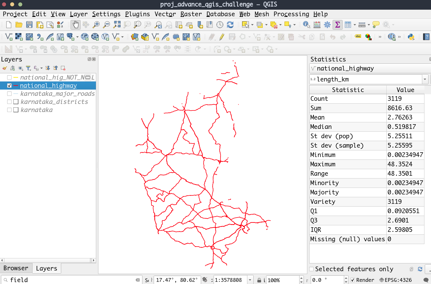
Figure: Stats from national_highway layer
And to remove the NULL in the "name" attribute:
"name" is NULL
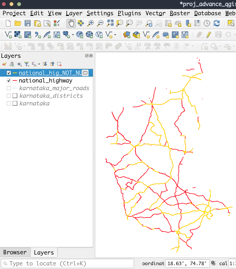
Figure: Solution day 2
Day 3 and 4
Challenge: Organizing the Attribute Table and processing algorithms
Calculate the length of national highways for each district in the state. This will require us to perform a spatial join and analyze the results using group statistics. Original solution (with tool box):
- Join attributes by Location
- Feature key: intersect
- Join type: For the Join type, you have 3 options. Here we want to do a one-to-one join where the for each road feature, we want to select one district feature. Select the Take attributes of the feature with largest overlap only option.
- Statistic by Categories
- Save the layer to the karnataka.gpkg as a layer named
national_highways_by_districts
Finally, the challenge: Apply the following formatting changes on the national_highways_by_districts layer and save it to karnataka.gpkg as a new layer national_highways_by_districts_formatted.
- Rename the DISTRICT field to district.
- Rename the sum field to total_length.
- Round the lengths in the total_length field to nearest integer using the round() function.
- Delete all remaining fields.
For all above steps, its possible to use processing algorithm called Refactor Fields. I use DB manager instead:
select national_highway.fid, karnataka_districts.DISTRICT AS 'district',
 round(sum(national_highway.length_km),0) AS 'total_lenght_km'
from national_highway, karnataka_districts
where (st_intersects (national_highway.geometry, karnataka_districts.geometry) )
group by karnataka_districts.DISTRICT
order by national_highway.fid
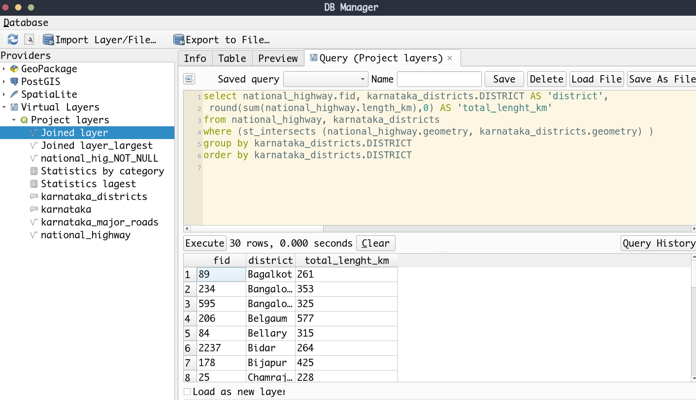
Figure: Solution day 3 by means DB manager
Note: In this query, the join type was: Create separate feature for each matching featura (one-to-many)
An alternative for the toll box Statistics by Categories is another tool called Execute SQL:
select DISTRICT, sum(length_km)
from input1
group by DISTRICT
Make sure to set Geometry type option as Mo geometry
Day 5
Batch Processing
All algorithms (including models) can be executed as a batch process. That is, they can be executed using not just a single set of inputs, but several of them, executing the algorithm as many times as needed. This is useful when processing large amounts of data, since it is not necessary to launch the algorithm many times from the toolbox.
To execute an algorithm as a batch process, right-click on its name in the toolbox and select the Execute as batch process option in the pop-up menu that will appear. Further details are available here.
Challenge: Re-projecting Multiple Layers by means Batch Processing
The challenge is Reprojected all the clipped layers to a UTM projection. You can reproject all the layers to the CRS WGS84 / UTM zone 43N EPSG:32643. Save the reprojected layers to the same GeoPackage clipped.gpkg
Steps:
- Cut layers by mask (
natural_earth_india — state_boundary) - Reproject by means batch processing
- Save all reproject layers in the same
Geopackage. For this, find in processing toolsPackage layers.
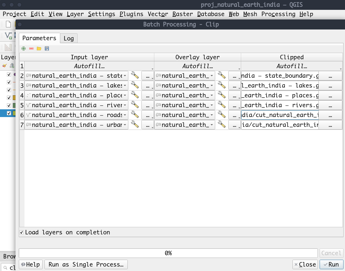
Figure: Partial solution:screen to cut layers with mask by means batch processing
The files .gpkg-shm and gpkg-wal are temporary files. It disappear after closed.
Day 6 and 7
Review and catch up on Week1 materials
…
Day 8
Using “Calculate by Expression” Autofill QGIS Easter Egg “bored”!
- Egg Easter: load a raster and type
boredin coordinates box, then press Enter . You got a puzzle.
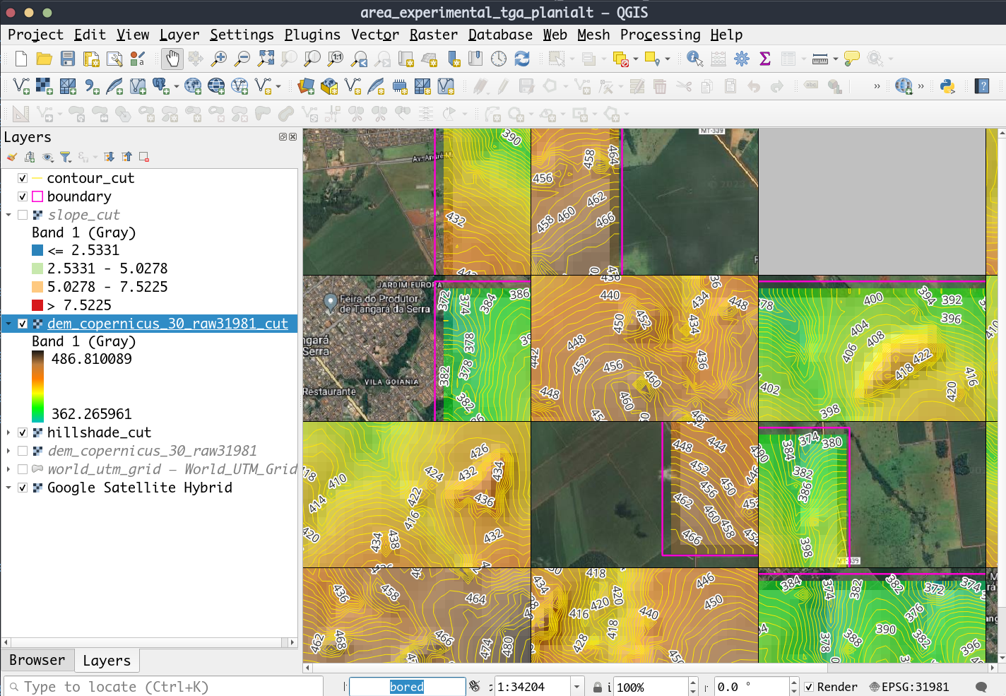
Figure: QGIS Puzzle by means *bored* egg Easter
- Calculate by Expression: Regarding the
Batch Processing, it is possible to use anExpressionto save the output file.
Day 9
QGIS Model Designer
The model designer allows you to create complex models using a simple and easy-to-use interface. When working with a GIS, most analysis operations are not isolated, rather part of a chain of operations. Using the model designer, that chain of operations can be wrapped into a single process, making it convenient to execute later with a different set of inputs. No matter how many steps and different algorithms it involves, a model is executed as a single algorithm, saving time and effort. The model designer can be opened from the Processing menu (Processing Model Designer) (This paragraph is from QGIS user manual).
The step by step to build this model is available on SpatialToughts.
Challenge: Extracting the Feature with the Highest Value
The challenge was extract the geometry (hexagon) with the greatest number of occurrences (count).
To solve it, an algorithm Extract by expression was add to filter values from Count_points_in_polygon. Thus the Input layer was Count_points_in_polygon, the Expression was "NUMPOINTS" = maximum( "NUMPOINTS" ), and the Matching features was assigned as MAX.
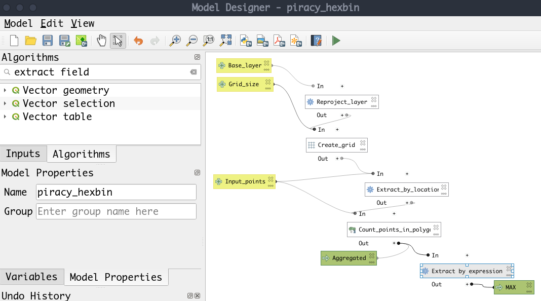
Figure: Model designer to extract Highest Value
Notice that maximum( "NUMPOINTS" ) just returns the maximum Value (NUMPOINTS). So it is necessary to select the feature(s) with the same value of the maximum NUMPOINTS.
The result on canvas:
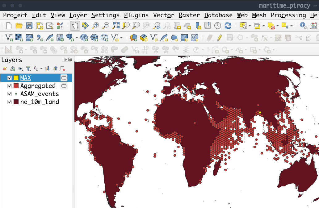
Figure: Solution from model designer
The exactly same process can be done by means python QGIS algorithm.
Day 10
Concept: Spatial Indexing Using Spatial Index
Running the Model (Piracy_hexbin) in the Day 9 we noticed a message as follow:
No spatial index exists for input layer, performance will be severely degraded Model processed OK. Executed 5 algorithms total in 7.878s. Execution completed in 7.89 seconds
There is no spatial index in the model, generating this error or warning. Thus it is necessary to create a spatial index, it can improve the processing time, specially for large operations.
A spatial index is a data structure that enables efficient querying and retrieval of spatial data, such as points, lines, and polygons in a multidimensional space. It is commonly used in geographic information systems (GIS), databases, and other applications that deal with spatial information MapScapping. In other words, a spatial index is a kind of extended index that to provide to index a spatial column (e.g. a column with geometry data)
From PostGis, a short explanation:
Standard database indexes create a hierarchical tree based on the values of the column being indexed. Spatial indexes are a little different – they are unable to index the geometric features themselves and instead index the bounding boxes of the features.
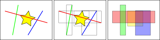
Figure: Spatial indexes
Off course, all the main concept is available on SpatialToughts.
Checking is a layer has Spatial Index:
$$
Properties => Source => Geometry
$$
The layer ASAM_events has Spatial index, otherwise the layer Aggregated has not. So, let’s return to Piracy_hexbin model and add the processing tool Create spatial index.
Note: The Geopackage file has spatial index by default.
The Spatial index will be between Create_grid and Extract Layer, as follow:
Standard database indexes create a hierarchical tree based on the values of the column being indexed. Spatial indexes are a little different – they are unable to index the geometric features themselves and instead index the bounding boxes of the features.
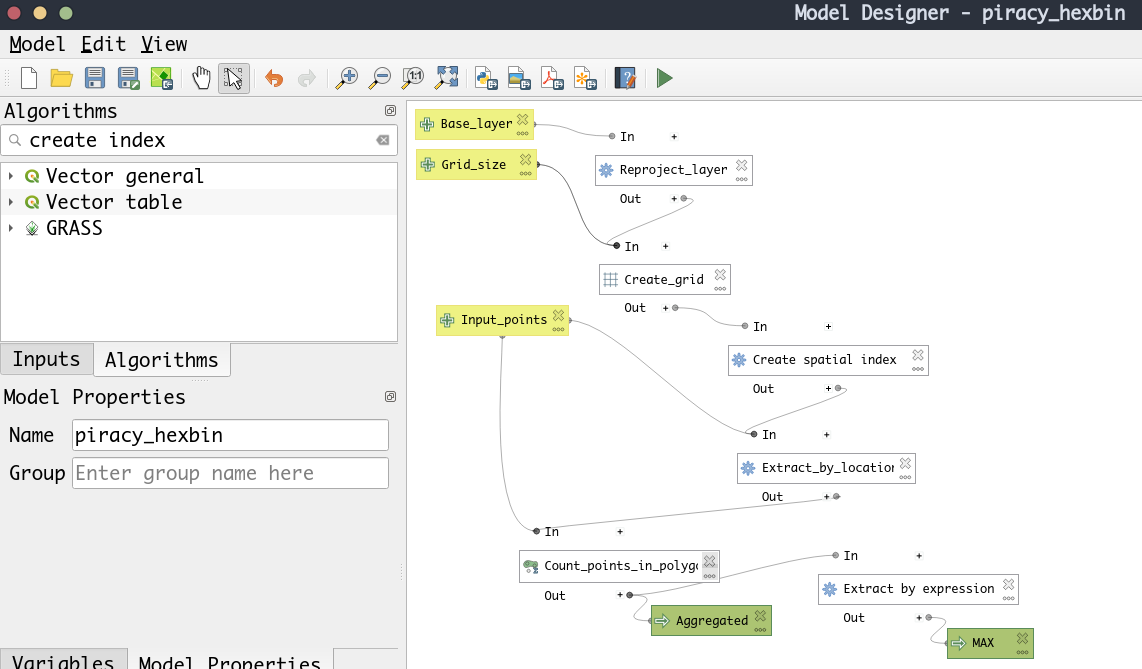
Figure: Spatial indexes
Now, the message on the log has changed, and the total time was around 10 time shorter:
Model processed OK. Executed 6 algorithms total in 0.786s. Execution completed in 0.81 seconds
Challenge: Converting Input Values in a Model
Challenge: Can you change the model so that instead of entering the grid size in meters, the user can enter the size in kilometers?
There are several options to solve it. One of them is to change in Create_grid the horizontal and vertical spacing. Initially there was the input Value as option, to transform the input from km to m, now you may use Pre-calculated Value instead. Finally, add the expression:
@grid_size_km * 1000
, as follow:
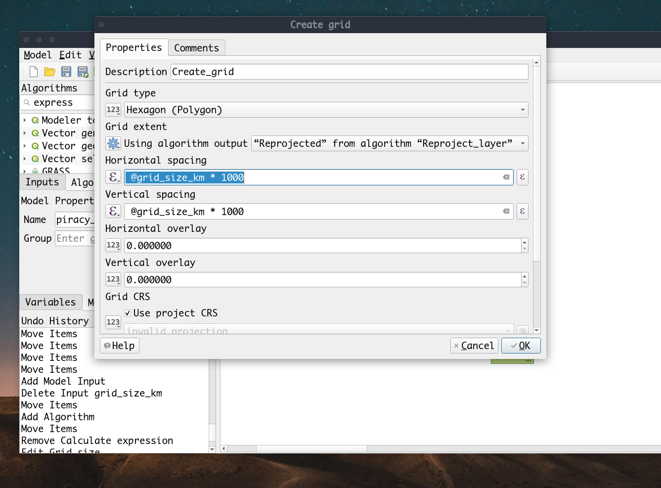
Figure: Algorithm Create Grid with Pre-calculated Value input
Day 11
Enabling Reproducible Workflows Concept: Understanding User Profiles
GeoPackage is an open and flexible data format that makes data management simple. We saw how you can package multiple layers in a GeoPackage. We will now learn how to embed QGIS projects inside of a goepackage.
QGIS projects contain information of layer configuration, symbology, label positions and even models. We can make the reproducing your workflow even easier by embedding the QGIS Project in the same geopackage containing the source layers.
-
Now, lets save this project in martime_piracy.gpkg geopackage. Click Project → Save To → GeoPackage….
-
In the Save project to GeoPackage dialog box, click … to browse to martime_piracy geopackage.
-
Enter project name as martime_piracy and click OK.
-
Now in Browser, under martime_piracy.gpkg the project is saved. You now have just 1 GeoPackage file that contains all your input layers, styles, project and models. Sharing this 1 file will enable anyone to reproduce your output using the embedded model and layers.
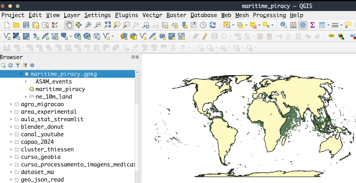
Figure: Project and files in a geopackage
Tip: Docking Attribute Table
Docking attribute table is very useful, because it makes easier to manage (close) the tables. In the menu Settings => Options => data sources , click on Open attribute table as docked window.
Day 12
Conditional Branch and Modeler Tools Assignment
A key feature introduced in QGIS 3.14 was the ability for models to have a conditional branch. This allows models to check for a condition and execute a different part of the model based on the output of the condition. This is equivalent to If/Else statements in a programming language.
Let us develop a Conditional branch in the piracy_hexbin model covered in the previous section. We will add a new check-box input Use Spatial Index - that allows the user to specify whether to use a spatial index in the model. We will add a conditional branch that takes the following actions:
If the Use Spatial Index option is selected, the model will create a spatial index for the grid layer and use it in the subsequent steps. If the option is not selected, the model will proceed without generating a spatial index.
Day 13 and 14
Weekend: Review and catch up on Week2 materials
Day 15
Assignment (continued from Day 12)
Your task is to create a model called Calculate Highway Statistics that will automate the workflow outlined in the previous section 1. Using Processing Toolbox.
Your model is expected to take following 3 inputs:
- Roads Layer: A vector layer of the road network. i.e. karnataka_major_roads.
- Admin Boundaries Layer: A vector layer containing admin boundaries. i.e. karnataka_districts
- Highway Type: An enum input with 2 options: National Highway and State Highway.
Steps to solve:
- Input Vector Layer for
MajorRoads - Input Enum to choose between National ou State road
- Algorithm Extract by expression to filter
MajorRoadsbased on Enum:
if( @highway_tyype = 0,
  regexp_match("ref", '^NH.*'),
  regexp_match("ref", '^SH.*')
  )
- Input Vector Layer
Districts - Algorithm Join Attributes by location:
DistrictsvsOutputfrom Extract from expression - Statistics by categories from output Join Attributes by location , vars
lenght_kmDISTRICT
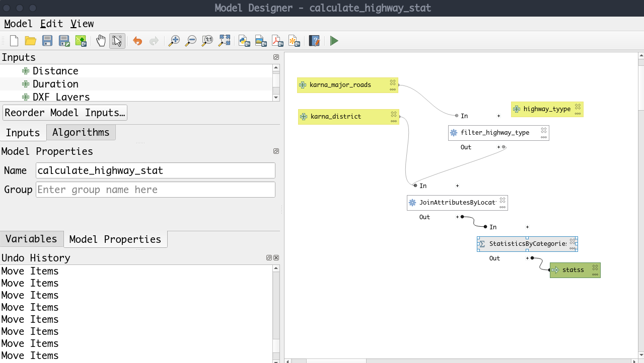
Figure: Assignment for Model Designer
QGIS Easter Egg ‘dizzy’
Type dizzy in coordinate label to shake the screen. It is a prank! To spot it is necessary to type dizzy again.
Day 16
- Rendering Map Layouts from a Model
Day 17
- 2D Animations
Challenge: Assigning Weights in a Heatmap
To create rules, we can use the Field Calculator:
CASE
WHEN  "hostilit_D" = 'Suspicious Approach' THEN 1
WHEN  "hostilit_D" = 'Kidnapping' THEN 2
WHEN  "hostilit_D" = 'Pirate Assault' THEN 5
WHEN  "hostilit_D" = 'Naval Engagement' THEN 10
ELSE 1
END
After just apply Heat Map in Layer Styling:
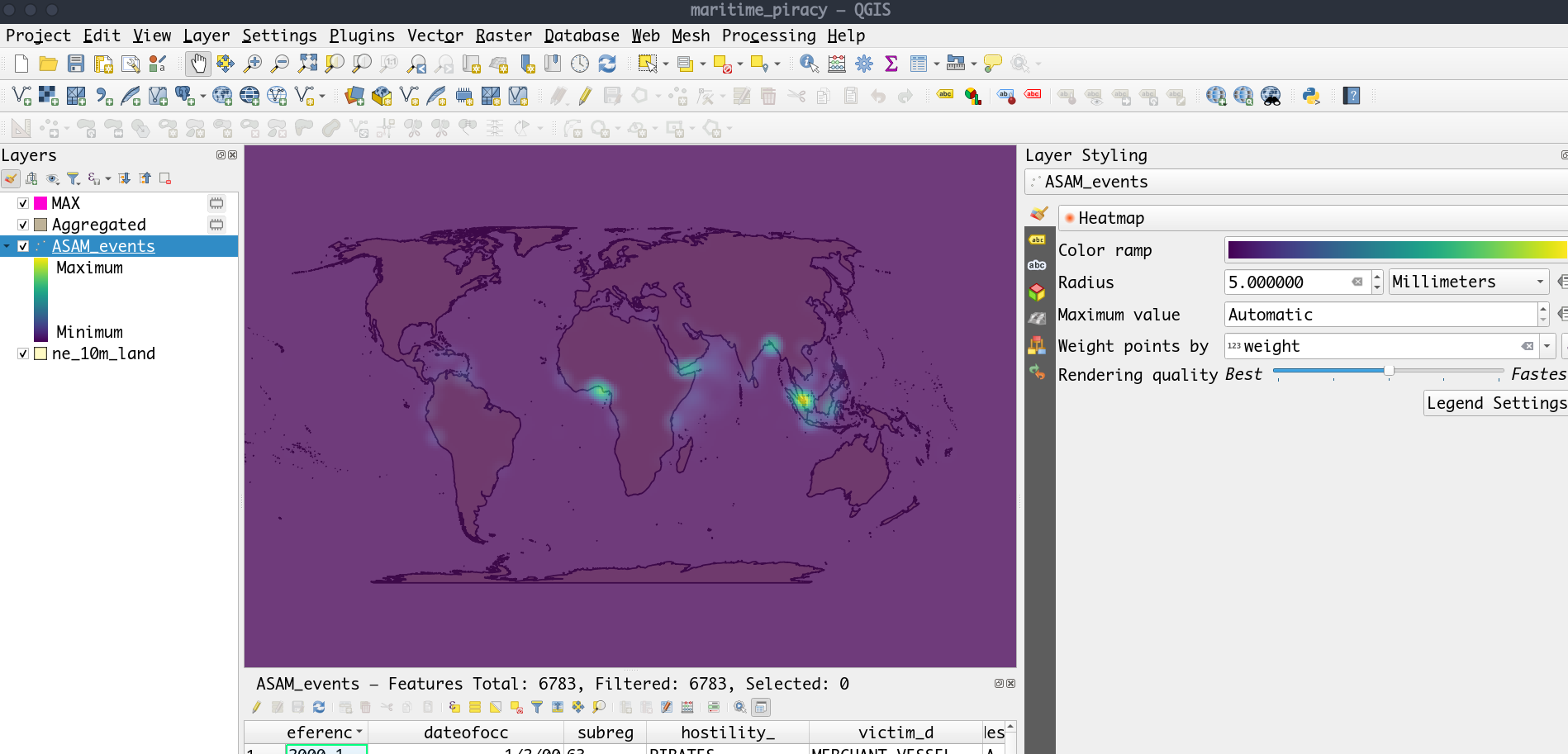
Figure: Heat map for an assigned weight
For the animation by means temporal date, in properties click on Temporal. Select the configuration, limits and the Field with the timestamp and click OK. If all was good, a clock will show on right side of the layer (Panel Layer). Now, We need to look for a icon with a clock to activate the Temporal Controler. Set the date range of the animation and play. To show the year or any text on the canvas click on menu View -> Decorator -> Title Label and apply an expression year(@map_start_time).
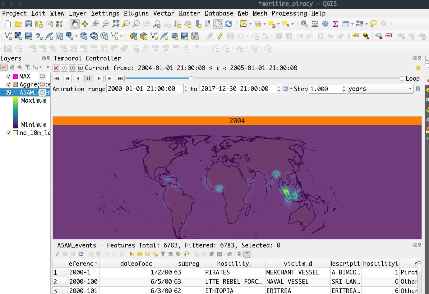
Figure: Heat map for an assigned weight
Day 18
- Exporting 2D Animation
To export these as images and convert them as GIF select the Export Animation (save icon) in the temporal controller window. It will export a lot of frames (figures) in .png format. Save all this frames in a folder. BEFORE exportation, make sure that the zoom in the canvas is as you wish.
In this example 18 frames were created:
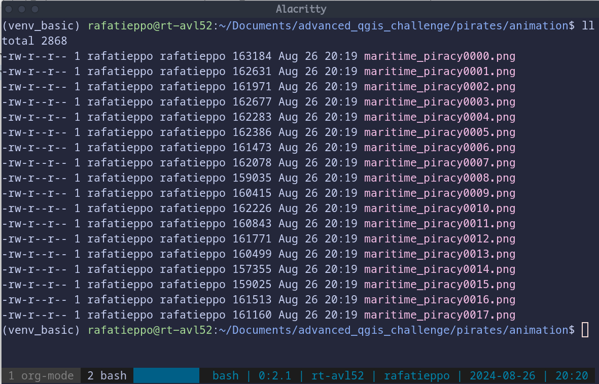
Figure: All 18 frames in png format
Now it is possible to use this frames in your favorite tool to generate the animation (.gif). One option is the site (https://ezgif.com/maker)[https://ezgif.com/maker] , and another on is to use the ImageMagick.
convert -size 1080x1080 -delay 100 -loop 0 *.png output.gif
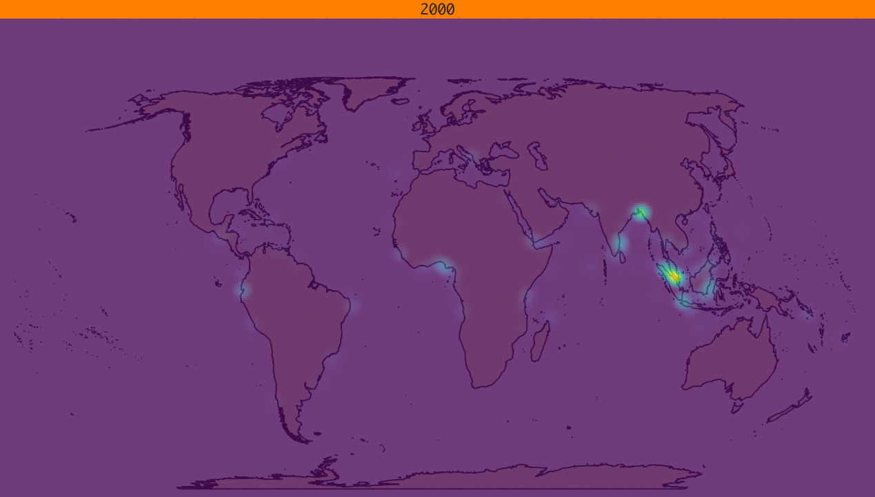
Figure: Animation (gif) from the generated frames.